
25 ChatGPT-5.5 Prompts for Data Scientists: Exploratory Data Analysis, Feature Engineering, and Model Evaluation

Why ChatGPT-5.5 Is a Game-Changer for Data Science Workflows
Data science has always been a discipline that rewards those who iterate quickly, document rigorously, and communicate findings clearly. ChatGPT-5.5 brings a qualitative leap to each of these dimensions — not just as a code generator, but as a reasoning partner capable of understanding the statistical nuances behind exploratory analysis, the tradeoffs inherent in feature engineering decisions, and the domain-specific context that separates a mediocre model from a production-ready one.
What makes these prompts different from generic AI prompts is their use of structured context variables — placeholders like [DATASET_NAME], [TARGET_VARIABLE], and [BUSINESS_CONSTRAINT] — that let you swap in your actual project details and receive output that feels authored, not hallucinated. Each prompt is engineered to extract the maximum analytical value from ChatGPT-5.5’s extended reasoning window and its improved ability to hold statistical context across multi-step analyses.
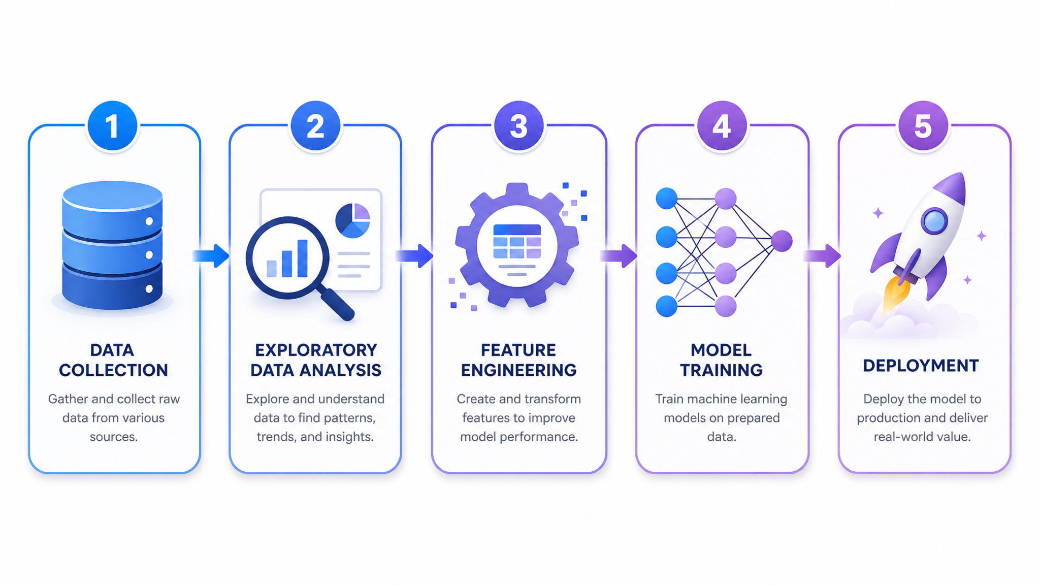
The 25 prompts in this guide are organized into five critical phases of the machine learning lifecycle: Exploratory Data Analysis, Feature Engineering, Model Selection and Training, Model Evaluation and Interpretation, and Production ML Pipeline. Whether you’re a solo data scientist working on a startup’s churn prediction model or part of a team building fraud detection infrastructure at scale, these prompts are designed to compress days of work into focused, actionable sessions with ChatGPT-5.5.
For those new to using language models in technical workflows, it’s worth noting that prompt quality directly determines output quality. Vague prompts produce vague answers. The prompts here are deliberately verbose because they front-load the context that ChatGPT-5.5 needs to produce expert-level output — and that verbosity pays dividends in precision and relevance. ChatGPT for Data Science Workflows
Section 1: Exploratory Data Analysis Prompts
Exploratory Data Analysis is the foundation of every sound modeling effort. Rushing past EDA is the most common source of downstream modeling failures — from misunderstood distributions to hidden data leakage. These five prompts are designed to turn ChatGPT-5.5 into a rigorous EDA collaborator that asks the right questions before touching a single algorithm.
Prompt 1: Comprehensive Dataset Audit and Quality Report
You are a senior data scientist conducting a thorough dataset audit before any modeling work begins.

Dataset context:
- Dataset name: [DATASET_NAME]
- Number of rows: [ROW_COUNT]
- Number of columns: [COLUMN_COUNT]
- Domain: [DOMAIN, e.g., "healthcare claims", "e-commerce transactions"]
- Target variable: [TARGET_VARIABLE]
- Task type: [CLASSIFICATION / REGRESSION / CLUSTERING]

Here is a sample of the data schema with column names and data types:
[PASTE SCHEMA OR FIRST 5 ROWS HERE]

Please perform a comprehensive dataset audit covering:

1. **Data quality assessment**: Identify columns with missing values above 5%, 20%, and 50% thresholds and recommend handling strategies for each tier.
2. **Cardinality analysis**: Flag high-cardinality categorical columns (>50 unique values) and low-cardinality numerical columns that may be miscoded categoricals.
3. **Target variable analysis**: Describe the distribution of [TARGET_VARIABLE], compute class imbalance ratio if classification, and flag if resampling strategies are warranted.
4. **Temporal integrity check**: If any datetime columns exist, verify monotonicity, identify gaps, and flag potential train/test leakage risks.
5. **Duplicate and near-duplicate detection strategy**: Recommend a Python-based approach (using pandas and hashlib) to detect exact and fuzzy duplicates.
6. **Schema anomalies**: Identify columns where inferred dtype differs from semantic meaning (e.g., zip codes stored as integers).

Output format: Provide findings as a structured report with a summary table showing column name, issue type, severity (Low/Medium/High), and recommended action. Then provide Python code snippets for each actionable finding.
When to use this prompt: Use this as the absolute first step when receiving a new dataset from a client, a data engineer, or a public repository. It replaces the ad-hoc df.info() / df.describe() workflow with a systematic audit that surfaces non-obvious issues — particularly the dtype mismatches and temporal leakage risks that junior analysts routinely miss. Run this before committing to any feature engineering direction.
Prompt 2: Univariate Distribution Analysis with Statistical Tests
You are a statistician-level data analyst. I need a rigorous univariate analysis of my numerical features.

Context:
- Dataset: [DATASET_NAME]
- Number of numerical features: [N_NUMERICAL]
- Sample size: [ROW_COUNT]
- Downstream model family: [LINEAR / TREE-BASED / NEURAL NETWORK]

For each numerical feature, generate a Python analysis script that:

1. Computes skewness and kurtosis, interpreting values relative to normality thresholds (skew > |1|, kurtosis > 3).
2. Applies the Shapiro-Wilk test (n < 5000) or D'Agostino-Pearson test (n ≥ 5000) for normality, adjusting for multiple comparisons using Bonferroni correction.
3. Detects outliers using three methods: IQR method, Z-score (threshold=3), and Isolation Forest — then produces a consensus outlier flag.
4. Visualizes each distribution using a 2x2 subplot: histogram with KDE, Q-Q plot, box plot, and ECDF.
5. Based on the [DOWNSTREAM MODEL FAMILY], recommends whether transformation (log, Box-Cox, Yeo-Johnson) is warranted and generates transformed versions with before/after normality test results.

Also produce a summary DataFrame with columns: [feature_name, n_missing, skewness, kurtosis, normality_test, p_value, n_outliers_iqr, n_outliers_zscore, n_outliers_iforest, recommended_transform].

Output all code as a single executable Python script using pandas, scipy, sklearn, and matplotlib/seaborn. Include docstrings for each function.
When to use this prompt: Deploy this prompt during the second phase of EDA, after the initial audit. It’s particularly valuable when preparing features for linear models or SVMs where distribution assumptions matter, and equally useful for tree-based models where extreme outliers can dominate split decisions. The consensus outlier detection — combining IQR, Z-score, and Isolation Forest — prevents the over-flagging that occurs when relying on any single method.
Prompt 3: Multivariate Correlation and Collinearity Analysis
Act as a senior machine learning engineer analyzing feature interdependencies.

Dataset details:
- Feature set size: [N_FEATURES] columns
- Mix of feature types: [N_NUMERICAL] numerical, [N_CATEGORICAL] categorical, [N_BINARY] binary
- Target: [TARGET_VARIABLE] ([TASK_TYPE])
- Concern level for multicollinearity: [HIGH / MEDIUM / LOW] (based on intended model type)

Please generate a comprehensive multivariate analysis covering:

1. **Pearson and Spearman correlation matrices** for numerical features — render as an annotated heatmap, highlighting pairs with |r| > 0.85 as high-collinearity candidates for removal or PCA consolidation.

2. **Variance Inflation Factor (VIF) analysis**: Compute VIF for all numerical features and flag anything above VIF=5 (moderate) and VIF=10 (severe). Provide a sequential VIF elimination procedure.

3. **Cramér's V matrix** for categorical feature pairs — interpret association strength using standard thresholds (0.1=weak, 0.3=moderate, 0.5=strong).

4. **Point-Biserial correlation** for numerical vs. binary feature pairs.

5. **Target correlation ranking**: Rank all features by their correlation/association with [TARGET_VARIABLE] — using the appropriate metric per feature type — and produce a ranked importance table.

6. **Redundancy cluster analysis**: Use hierarchical clustering on the correlation matrix to identify feature clusters, recommending one representative feature per cluster where correlation exceeds 0.90.

Output: Python code using pandas, scipy, statsmodels, seaborn, and sklearn. Also produce a written interpretation of the three most critical multicollinearity findings and their recommended resolutions.
When to use this prompt: Critical for any regression task where multicollinearity inflates standard errors and distorts coefficient interpretations. Also essential before deploying SHAP values on models trained with highly correlated features, where attribution can be misleading. The Cramér’s V extension is especially useful for datasets heavy in categorical features — insurance, healthcare, and HR datasets where one-hot encoding can explode dimensionality.
Prompt 4: Target Leakage Detection Framework
You are a machine learning engineer specialized in data pipeline integrity. Your task is to systematically audit a feature set for target leakage — one of the most common causes of deceptively high model performance that collapses in production.

Project context:
- Dataset: [DATASET_NAME]
- Target variable: [TARGET_VARIABLE]
- Prediction timing: The model will be invoked at [PREDICTION_POINT, e.g., "time of loan application", "24 hours before customer churn event"]
- Data collection process: [BRIEF DESCRIPTION OF HOW DATA IS COLLECTED]
- Known high-risk features: [LIST ANY FEATURES YOU SUSPECT, OR "UNKNOWN"]

Perform a leakage audit covering:

1. **Temporal leakage**: Identify any features that could only be known AFTER the event defined by [TARGET_VARIABLE] occurs. Generate a timeline diagram (ASCII format) showing feature availability at [PREDICTION_POINT].

2. **Proxy leakage**: Use mutual information scores to flag features with suspiciously high MI scores relative to [TARGET_VARIABLE] (threshold: MI > 0.5 for binary targets). For each flagged feature, reason through whether the information could plausibly be available at prediction time.

3. **ID-style leakage**: Check for columns that appear to be identifiers but encode target information (e.g., sequential IDs assigned after a decision, status codes updated post-event).

4. **Aggregation leakage**: If any features are pre-computed aggregates (e.g., "average order value"), verify that aggregations are computed only on historical data relative to each row's timestamp.

5. **Split contamination check**: Recommend a validation protocol — including time-based splits if temporal data exists — that prevents any form of future information from entering training folds.

Output: A leakage risk matrix (feature name, leakage type, risk level, reasoning, recommended action) and Python code for automated MI-based leakage screening.
When to use this prompt: Use this prompt before every model training run on a new dataset, and again whenever a model’s cross-validation AUC seems unusually high (above 0.95 for real-world business problems). Target leakage is epidemic in financial services, healthcare readmission models, and customer churn prediction — domains where data engineers often include features computed from post-event records. Preventing Data Leakage in Machine Learning
Prompt 5: Segment-Level EDA for Population Heterogeneity
You are a senior data scientist conducting stratified EDA to understand whether a single global model is appropriate or whether separate models per segment would be more effective.

Dataset context:
- Dataset: [DATASET_NAME]
- Target: [TARGET_VARIABLE]
- Candidate segmentation variables: [LIST VARIABLES, e.g., "region", "customer_tier", "product_category"]
- Business constraint: [DESCRIBE, e.g., "we must use a single model per regulatory requirement" or "separate models per segment are acceptable"]

Conduct a segment-level analysis:

1. **Segment size and balance**: Compute the distribution of rows across each segment variable. Flag segments with fewer than [MIN_SEGMENT_SIZE, e.g., 500] rows as potentially unreliable for separate modeling.

2. **Target rate heterogeneity**: Compute the target event rate per segment. Perform chi-square tests (classification) or ANOVA/Kruskal-Wallis (regression) to determine if target distributions differ significantly across segments.

3. **Feature importance variation by segment**: Train a shallow decision tree (max_depth=3) per segment and compare top feature importances. Identify cases where the most predictive feature changes across segments — a strong signal for interaction effects.

4. **Distribution shift detection**: For the top 10 features by overall importance, compute the Population Stability Index (PSI) between each pair of segments. Flag PSI > 0.2 as a meaningful shift.

5. **Interaction effect hypothesis generation**: Based on findings, propose the top 5 interaction features (e.g., feature_A × segment_flag) that could improve a global model's performance on heterogeneous data.

Output: A segment analysis report with visualizations (grouped bar charts, faceted distribution plots), a PSI table, and Python code using pandas, scipy, sklearn, and matplotlib.
When to use this prompt: Essential when business stakeholders ask “should we build one model or multiple models per region/product/customer type?” This prompt replaces days of ad-hoc segmentation analysis with a structured framework that produces defensible, data-driven answers. Particularly valuable in retail banking, insurance underwriting, and multi-market e-commerce contexts.
Section 2: Feature Engineering Prompts
Feature engineering remains the highest-leverage activity in applied machine learning — a discipline where domain knowledge, mathematical creativity, and systematic experimentation intersect. These five prompts are designed to help you extract maximum signal from raw data, whether you’re working with tabular records, time series, or text-enriched datasets.
Prompt 6: Automated Feature Construction for Tabular Data
You are a feature engineering specialist with expertise in tabular machine learning competitions and production ML systems.

Dataset context:
- Dataset: [DATASET_NAME]
- Feature types available: [LIST, e.g., "5 numerical continuous, 3 categorical ordinal, 2 categorical nominal, 1 datetime, 1 free-text"]
- Target: [TARGET_VARIABLE] ([TASK_TYPE])
- Downstream model: [MODEL_TYPE, e.g., "LightGBM", "Logistic Regression", "Neural Network"]
- Compute budget: [LOW / MEDIUM / HIGH] (affects complexity of features generated)

Generate a comprehensive feature engineering plan covering:

1. **Numerical feature transformations**: For each numerical feature, generate: log(x+1), sqrt(x), x², 1/x (with zero-guard), and binned versions (equal-width and equal-frequency with 5, 10 bins). Include a selection criterion based on correlation gain with target.

2. **Ratio and interaction features**: Systematically generate pairwise ratios (A/B) and products (A×B) for all numerical pairs. Use mutual information with target to select the top 20 generated features.

3. **Datetime feature extraction**: From [DATETIME_COLUMN], extract: year, month, day, day_of_week, hour, is_weekend, is_month_end, days_since_epoch, cyclic encoding (sin/cos) for month and hour.

4. **Categorical encoding strategy**: Based on cardinality and downstream model type, recommend and implement: one-hot encoding (cardinality < 10), target encoding with leave-one-out cross-validation (cardinality 10–50), frequency encoding (cardinality > 50), and hash encoding (cardinality > 200).

5. **Text feature extraction** (if applicable): From [TEXT_COLUMN], generate: character count, word count, sentence count, average word length, punctuation density, TF-IDF top-20 terms, and sentiment score using VADER.

6. **Feature selection post-construction**: After generating all features, apply a two-stage filter — (1) remove features with near-zero variance (threshold=0.01), (2) remove features with pairwise correlation > 0.95 using a greedy elimination approach.

Output: Complete Python code as a reusable FeatureEngineer class with fit() and transform() methods compatible with sklearn pipelines.
When to use this prompt: Use when starting feature engineering on a new dataset, especially for tabular competitions or when a business stakeholder has provided raw transactional or behavioral data with minimal pre-processing. The sklearn-compatible output is critical for teams who need reproducible, pipeline-ready feature transformations that won’t leak in cross-validation.
Prompt 7: Time Series Feature Engineering for Forecasting and Classification
Act as a time series machine learning expert. I need to engineer features from temporal data for a [FORECASTING / CLASSIFICATION] task.

Dataset context:
- Time series identifier column: [ID_COLUMN, or "single series"]
- Timestamp column: [TIMESTAMP_COLUMN]
- Value column(s): [VALUE_COLUMNS]
- Sampling frequency: [FREQUENCY, e.g., "daily", "hourly", "5-minute"]
- Forecast horizon (if forecasting): [HORIZON]
- History available per entity: [MIN_HISTORY_LENGTH] to [MAX_HISTORY_LENGTH] periods
- External regressors available: [LIST OR "NONE"]

Generate a time series feature engineering pipeline covering:

1. **Lag features**: Generate lags at [1, 2, 3, 7, 14, 28] periods (adjusted for [FREQUENCY]). Include a lag validity mask to flag rows where insufficient history exists.

2. **Rolling statistics**: Compute rolling mean, std, min, max, median, skewness, and kurtosis over windows of [WINDOW_SIZES, e.g., "7, 14, 30, 90"] periods. Use expanding window variants for the first N periods.

3. **Exponential weighted features**: Apply EWM with spans [3, 7, 14, 30] to capture trend with recency weighting. Compute EWM mean, EWM std, and rate-of-change of EWM mean.

4. **Trend and seasonality decomposition**: Apply STL decomposition (statsmodels) and use trend, seasonal, and residual components as features. Compute residual anomaly score (residual / rolling_std).

5. **Cross-series features** (if panel data): Compute rank of each entity's current value relative to the population at each timestamp. Compute z-score relative to population mean/std per timestamp.

6. **Target encoding for time series**: For the [CLASSIFICATION] task variant, compute the historical event rate per entity with an expanding window to prevent leakage.

Output: A Python pipeline using pandas, numpy, statsmodels, and tsfresh (optional), with built-in leakage prevention via proper time-aware windowing. Include unit tests for lag validity and rolling window correctness.
When to use this prompt: The most common source of errors in time series modeling is lag feature leakage — rolling statistics computed without proper time alignment. This prompt’s emphasis on leakage prevention and lag validity masks makes it invaluable for demand forecasting, anomaly detection, and predictive maintenance projects. Use it any time your data has a meaningful temporal structure.
Prompt 8: Domain-Specific Feature Engineering for [DOMAIN]
You are a machine learning engineer with deep expertise in [DOMAIN: e.g., "retail banking and credit risk", "healthcare and clinical outcomes", "e-commerce and customer behavior"].

Project context:
- Business problem: [DESCRIBE, e.g., "predict 90-day loan default probability"]
- Available raw data tables: [LIST TABLES, e.g., "transactions, account_info, credit_bureau, customer_demographics"]
- Granularity of modeling unit: [e.g., "one row per customer per month"]
- Key domain constraints: [e.g., "FCRA-compliant features only", "no use of protected attributes"]

Generate domain-specific feature engineering recommendations:

1. **Domain feature taxonomy**: Enumerate the canonical feature categories used in [DOMAIN] ML systems (e.g., for credit: utilization rate, payment velocity, derogatory marks, credit mix). For each category, generate the specific calculation from the available raw tables.

2. **Behavioral sequence features**: Design features that capture behavioral trajectories over the past [3, 6, 12] months — not just point-in-time snapshots. Examples: trend in monthly spend, acceleration in delinquency rate, recency-frequency-monetary (RFM) scoring.

3. **Interaction and ratio features from domain knowledge**: Generate 10 domain-informed feature interactions that an expert in [DOMAIN] would hypothesize — explaining the economic/clinical/behavioral rationale for each.

4. **Derived risk/propensity scores**: Where domain conventions exist (e.g., DTI ratio in banking, Charlson Comorbidity Index in healthcare), implement standard score calculations from raw fields.

5. **Regulatory/compliance feature audit**: Flag any proposed features that could constitute proxies for protected classes under [RELEVANT_REGULATION, e.g., "ECOA", "HIPAA", "GDPR"]. Suggest fairness-aware alternatives.

Output: A feature catalog as a Python dictionary mapping feature names to their calculation logic, plus SQL and pandas implementations for each feature.
When to use this prompt: Use when entering a new industry domain where feature engineering conventions are well-established but not immediately obvious. Providing ChatGPT-5.5 with the domain context and the raw table structure allows it to generate features that reflect genuine domain expertise — the kind that typically comes from years of experience working in that vertical. ChatGPT Prompts for Machine Learning Engineers
Prompt 9: Feature Importance-Guided Feature Selection Pipeline
You are a machine learning engineer building a rigorous, reproducible feature selection pipeline.

Context:
- Dataset: [DATASET_NAME]
- Feature count before selection: [N_FEATURES]
- Target: [TARGET_VARIABLE] ([TASK_TYPE])
- Primary model: [MODEL_TYPE]
- Target number of features: [TARGET_N_FEATURES, or "determine automatically"]
- Cross-validation strategy: [K-FOLD / STRATIFIED K-FOLD / TIME-SERIES SPLIT], k=[K]

Build a multi-stage feature selection pipeline:

Stage 1 — Filter Methods (model-agnostic):
- Variance threshold filter (remove features where variance < 0.01)
- Mutual information scores for all features vs. target
- ANOVA F-score (for numerical features with classification target)
- Chi-square test (for categorical features with classification target)
- Produce a ranking table combining all filter scores

Stage 2 — Wrapper Methods:
- Recursive Feature Elimination with Cross-Validation (RFECV) using [MODEL_TYPE] as estimator
- Forward sequential feature selection with early stopping
- Track validation score vs. number of features curve

Stage 3 — Embedded Methods:
- Train [MODEL_TYPE] with L1 regularization (or feature importance for tree models)
- Extract and rank feature importances / coefficients
- Apply stability selection: run 100 bootstrap iterations, compute selection frequency per feature

Stage 4 — Consensus Selection:
- Rank features by their average rank across all applicable methods
- Select features that appear in top-[TARGET_N_FEATURES] across at least 2 of 3 method categories
- Validate selected feature set: compare [MODEL_TYPE] performance with full feature set vs. selected set using [CV_STRATEGY]

Output: A SelectionPipeline class with fit/transform interface, a feature selection report with all intermediate rankings, and a plotted selection stability curve.
When to use this prompt: Deploy this when your feature set has grown large (50+ features) through prior engineering steps, or when model interpretability and inference speed are constraints. The stability selection component — often omitted in ad-hoc feature selection — is particularly important for production models where feature availability might vary and you need to understand which features are robustly predictive versus incidentally correlated in your training data.
Prompt 10: Embeddings and Representation Learning for High-Cardinality Categoricals
You are a deep learning engineer specializing in representation learning for tabular and semi-structured data.

Context:
- High-cardinality categorical column: [COLUMN_NAME] with [N_UNIQUE] unique values
- Column type: [e.g., "product SKU", "merchant category code", "user ID", "geographic location"]
- Row count: [ROW_COUNT]
- Downstream task: [TASK_TYPE] with target [TARGET_VARIABLE]
- Compute constraint: [GPU_AVAILABLE: YES/NO]

Design an embedding strategy for [COLUMN_NAME]:

1. **Entity embedding via neural network**: Build a PyTorch embedding network that learns entity embeddings jointly with the prediction task. Specify embedding dimension as min(50, (N_UNIQUE + 1) // 2). Include dropout (p=0.3) on embedding layers.

2. **Word2Vec-style co-occurrence embeddings**: If [COLUMN_NAME] appears in sequences (e.g., product purchase sequences, merchant visit sequences), train a Word2Vec or FastText model on sequences to produce behavioral embeddings. Specify window size and dimensionality based on [ROW_COUNT].

3. **Target-informed embeddings via CatBoost**: Use CatBoost's built-in categorical embedding — describe how it encodes categories using ordered target statistics and why it outperforms naive target encoding.

4. **Embedding quality evaluation**: Post-training, evaluate embedding quality using: (a) t-SNE / UMAP visualization with semantic coloring, (b) analogy test if semantic relationships exist (e.g., similar product categories should cluster), (c) downstream model performance comparison: raw target encoding vs. entity embedding vs. Word2Vec embedding.

5. **Embedding reuse strategy**: Package learned embeddings as a lookup table that can be injected into sklearn pipelines for inference without requiring the full neural network at prediction time.

Output: Complete PyTorch and sklearn-compatible Python code, plus a qualitative guide on choosing between the three embedding approaches for different column semantics.
When to use this prompt: Indispensable for recommendation systems, retail analytics, and any domain with high-cardinality entity columns (user IDs, product codes, merchant categories). Standard approaches like one-hot encoding are computationally infeasible at high cardinalities, while naive target encoding loses the semantic structure that embeddings can capture. This prompt bridges the gap between tabular ML and deep learning methodologies.
Section 3: Model Selection and Training Prompts
Choosing the right model architecture and training it correctly is where statistical knowledge, engineering discipline, and business understanding converge. These five prompts help you navigate model selection with rigor, implement hyperparameter optimization efficiently, and build training pipelines that are reproducible and production-aware from day one.
Prompt 11: Model Selection Framework Based on Problem Constraints
Act as a principal machine learning engineer advising on model selection. I need a structured framework to choose the optimal algorithm given my specific constraints.

Problem specification:
- Task type: [BINARY CLASSIFICATION / MULTICLASS / REGRESSION / RANKING / ANOMALY DETECTION]
- Dataset size: [ROW_COUNT] rows × [N_FEATURES] features
- Feature types: [DESCRIBE MIX]
- Target: [TARGET_VARIABLE], class balance: [BALANCE_RATIO or "balanced"]
- Primary metric: [AUC-ROC / F1 / RMSE / NDCG / etc.]
- Interpretability requirement: [NONE / FEATURE IMPORTANCE / FULL EXPLAINABILITY]
- Latency constraint at inference: [e.g., "<10ms p99", "batch OK", "real-time required"]
- Training frequency: [ONCE / WEEKLY RETRAIN / ONLINE LEARNING]
- Infrastructure: [CPU-ONLY / GPU AVAILABLE / CLOUD ML PLATFORM]

Produce a model selection analysis:

1. **Candidate model evaluation matrix**: Evaluate the following model families against all constraints above: Logistic/Linear Regression, Decision Tree, Random Forest, Gradient Boosted Trees (XGBoost, LightGBM, CatBoost), SVM, k-NN, Neural Network (MLP), and TabNet. Score each on a 1–5 scale per constraint with justification.

2. **Top-3 recommendation with rationale**: Recommend the top 3 models ranked by overall fit to the constraint profile. For each, explain: (a) why it fits the data characteristics, (b) known failure modes to monitor, (c) expected training and inference time at the given scale.

3. **Baseline model specification**: Define the simplest defensible baseline for this problem (e.g., majority class, mean predictor, rule-based heuristic) and specify how to compute it.

4. **Ensemble strategy**: If multiple models are recommended, design an ensemble (stacking/blending/voting) strategy and explain when it's worth the added complexity.

Output: A decision matrix table, ranked recommendations with prose justification, and a Python code template for training and evaluating all three recommended models with a unified evaluation harness.
When to use this prompt: Use at the start of the modeling phase, before writing any model-specific code. The constraint-driven evaluation matrix prevents the common mistake of defaulting to the “fashionable” algorithm (currently LLM-based or transformer architectures for tabular data) when a well-tuned LightGBM would outperform it at a fraction of the computational cost.
Prompt 12: Bayesian Hyperparameter Optimization Strategy
You are an ML engineer designing an efficient hyperparameter optimization strategy for a production model.

Model context:
- Model: [MODEL_TYPE, e.g., "LightGBM", "XGBoost", "Neural Network"]
- Training set size: [TRAIN_SIZE]
- Approximate training time per trial (full dataset): [TRIAL_TIME, e.g., "45 seconds"]
- Optimization budget: [MAX_TRIALS or MAX_WALL_TIME]
- Primary metric to optimize: [METRIC]
- Validation strategy: [K-FOLD / HOLDOUT / TIME-SERIES SPLIT]
- Framework preference: [Optuna / Hyperopt / Ray Tune / SMAC]

Design a hyperparameter optimization protocol:

1. **Search space definition**: For [MODEL_TYPE], define a comprehensive yet bounded search space. Include:
   - Parameter type (continuous log-scale, integer, categorical)
   - Recommended bounds based on dataset size and feature count
   - Parameter interactions that should be considered (e.g., learning_rate and n_estimators are inversely related)

2. **Pruning strategy**: Implement Optuna's MedianPruner or HyperbandPruner to terminate unpromising trials early. Specify warmup_steps appropriate for the dataset size.

3. **Multi-fidelity optimization**: Design a two-phase approach — (Phase 1) coarse search on 20% of training data with 100 trials; (Phase 2) fine search on full data with top-10 parameter regions, 30 trials.

4. **Overfitting guard**: Add a constraint that the optimization objective penalizes large train/validation gaps: objective = val_metric - max(0, train_metric - val_metric - [TOLERANCE])

5. **Results analysis**: After optimization, generate: (a) parameter importance plot using fANOVA, (b) parallel coordinate plot of all trials, (c) optimization history plot, (d) final recommended hyperparameters with confidence intervals from top-10 trials.

Output: Complete Optuna study code (or [FRAMEWORK_PREFERENCE] equivalent), a hyperparameter specification table with bounds and rationale, and a post-optimization analysis notebook.
When to use this prompt: When grid search is too slow and random search isn’t structured enough. The multi-fidelity approach (early exploration on subsets, refinement on full data) typically reduces optimization wall time by 60-80% compared to naive Bayesian optimization on the full dataset. Critical for teams with GPU or cloud compute budgets.
Prompt 13: Imbalanced Learning Strategy for Rare Event Detection
You are a machine learning researcher specializing in imbalanced learning. My dataset has significant class imbalance and I need a rigorous strategy to build a high-performance rare event detector.

Problem context:
- Task: Binary classification
- Dataset size: [ROW_COUNT]
- Class ratio (minority:majority): 1:[IMBALANCE_RATIO, e.g., "1:100", "1:500"]
- Domain: [DOMAIN, e.g., "fraud detection", "medical diagnosis", "equipment failure"]
- Business priority: [MAXIMIZE RECALL / MAXIMIZE PRECISION / MAXIMIZE F1 / CUSTOM THRESHOLD]
- False negative cost vs. false positive cost ratio: [COST_RATIO, e.g., "10:1"]
- Base model: [MODEL_TYPE]

Design a comprehensive imbalanced learning strategy:

1. **Resampling methods comparison**: Implement and benchmark: SMOTE, ADASYN, BorderlineSMOTE, SMOTEENN (combined over+undersampling), and RandomUnderSampler. Use cross-validation (StratifiedKFold, k=5) to compare — critical: resampling must occur only within training folds.

2. **Algorithmic approaches**: Configure class_weight='balanced' and custom cost-sensitive weights derived from the [COST_RATIO]. For tree-based models, implement scale_pos_weight (XGBoost) or is_unbalance (LightGBM).

3. **Threshold optimization**: Post-training, optimize the classification threshold using: (a) F-beta score maximization (beta tuned to [COST_RATIO]), (b) precision-recall curve analysis, (c) cost-sensitive threshold via expected cost minimization using [COST_RATIO].

4. **Evaluation metrics for imbalance**: Replace accuracy with: AUC-ROC, AUC-PR (Average Precision), F-beta score, Matthews Correlation Coefficient (MCC), and G-mean. Explain why each is more informative than accuracy in this context.

5. **Ensemble of diverse strategies**: Build a stacking ensemble where base models are trained with different imbalance handling strategies — creates diversity that improves robustness.

Output: Python code using imbalanced-learn and sklearn, a benchmark table comparing all strategies on all evaluation metrics, and a decision guide for selecting the final approach based on [BUSINESS_PRIORITY].
When to use this prompt: Any time your minority class represents less than 10% of your dataset — which includes the majority of high-value business problems: fraud, medical events, equipment failures, and customer churn in healthy businesses. The emphasis on correct resampling placement within cross-validation folds is non-negotiable; applying SMOTE before splitting is a form of data leakage that inflates reported performance.
Access 40,000+ AI Prompts for ChatGPT, Claude & Codex — Free!
Subscribe to get instant access to our complete Notion Prompt Library — the largest curated collection of prompts for ChatGPT, Claude, OpenAI Codex, and other leading AI models. Optimized for real-world workflows across coding, research, content creation, and business.
Prompt 14: Cross-Validation Strategy Design for Non-IID Data
Act as a statistical learning theorist helping me design a validation strategy for data that violates the IID assumption.

Dataset characteristics:
- Data type: [TIME SERIES / PANEL DATA / SPATIAL DATA / HIERARCHICAL/GROUPED]
- Temporal ordering: [YES/NO]
- Group/entity column: [GROUP_COLUMN, or "N/A"]
- Spatial component: [DESCRIBE OR "N/A"]
- Dataset size: [ROW_COUNT]
- Approximate training time: [TRAINING_TIME]
- Target: [TARGET_VARIABLE]

Design an appropriate cross-validation framework:

1. **IID violation analysis**: Diagnose which IID assumptions are violated in this dataset. For time series: autocorrelation (ACF/PACF analysis). For grouped data: intra-class correlation coefficient (ICC). For spatial data: Moran's I statistic.

2. **Custom CV splitter implementation**: Based on the violation type, implement a custom sklearn-compatible cross-validator:
   - Time series: TimeSeriesSplit with purging (gap between train/test equal to prediction horizon) and embargoing (additional gap to prevent leakage from lookahead)
   - Grouped: GroupKFold ensuring all rows from one group are in same fold
   - Hierarchical: Custom splitter respecting cluster structure

3. **Backtesting for time series**: Implement a walk-forward validation with expanding and sliding window variants. Visualize all train/test splits to verify correctness.

4. **Nested CV for unbiased model selection**: When both feature selection and model evaluation need to happen, implement nested cross-validation (outer loop for evaluation, inner loop for HPO/feature selection).

5. **Variance of CV estimates**: Compute confidence intervals for CV score estimates using the Bates et al. corrected t-test for k-fold CV, which accounts for overlap between folds.

Output: Custom CV splitter class, visualization code for all splits, statistical analysis of IID violation severity, and a decision guide for interpreting CV scores in the presence of each violation type.
When to use this prompt: Standard k-fold cross-validation is incorrect for any dataset where rows are not independent — which includes time series, panel data, customer-level data (multiple rows per customer), and geographic data. The corrected variance estimates are particularly valuable when comparing two models and needing to determine if the performance difference is statistically meaningful. Advanced Cross-Validation Techniques for Time Series
Prompt 15: Multi-Objective Model Training with Business Constraints
You are a machine learning engineer translating business requirements into a multi-objective optimization problem.

Business context:
- Primary ML objective: Maximize [PRIMARY_METRIC, e.g., "AUC-ROC"]
- Business constraints (hard):
  * Minimum recall on positive class: [MIN_RECALL, e.g., 0.80]
  * Maximum FPR: [MAX_FPR, e.g., 0.05]
  * Maximum inference latency: [MAX_LATENCY, e.g., "5ms"]
  * Fairness constraint: Demographic parity difference < [FAIRNESS_THRESHOLD, e.g., 0.05] across [PROTECTED_ATTRIBUTE]
- Secondary objective: [e.g., "minimize model complexity (number of features used)"]
- Model family: [MODEL_TYPE]

Design a constrained multi-objective training framework:

1. **Constraint formalization**: Convert all business constraints into mathematical form. Define the feasible region in metric space.

2. **Pareto frontier exploration**: Use Optuna's multi-objective mode (directions=['maximize', 'minimize']) to explore the Pareto frontier between [PRIMARY_METRIC] and [SECONDARY_OBJECTIVE]. Visualize the frontier.

3. **Constraint-aware trial pruning**: During HPO, immediately prune trials that violate hard constraints (recall, FPR, latency). Implement as an Optuna callback.

4. **Fairness constraint implementation**: Compute demographic parity difference during each CV fold. Add as a hard constraint to the optimization — solutions violating fairness are infeasible regardless of predictive performance.

5. **Post-Pareto decision**: After generating the Pareto frontier, apply a weighted utility function to select the final model: utility = w1 × [PRIMARY_METRIC] + w2 × (1 - latency_score) - penalty × constraint_violations. Present sensitivity analysis of utility weights.

Output: Python code for constrained multi-objective optimization using Optuna, a Pareto frontier visualization, a final model selection summary with full constraint verification report.
When to use this prompt: Use when deploying models in regulated industries (lending, hiring, healthcare) where business and legal constraints create a multi-objective problem that pure metric maximization cannot address. The fairness constraint implementation is particularly relevant for ECOA compliance in credit models or EEOC compliance in HR applications.
Section 4: Model Evaluation and Interpretation Prompts
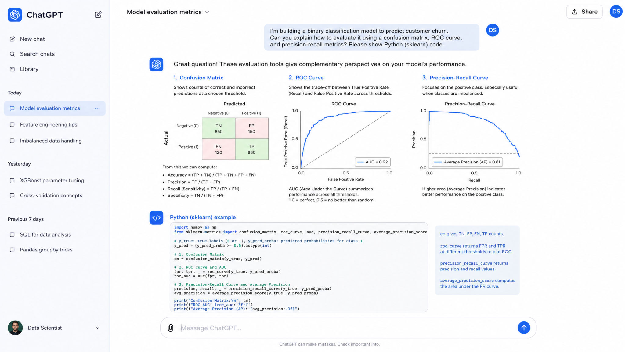
A model that cannot be explained to business stakeholders cannot be trusted, and a model that cannot be audited cannot be deployed responsibly. These five prompts build the evaluation and interpretability layer that transforms a trained model from a black box into a transparent, defensible business asset.
Prompt 16: Comprehensive Model Evaluation Report
You are a machine learning engineer preparing a rigorous model evaluation report for stakeholder review.

Model context:
- Model type: [MODEL_TYPE]
- Task: [TASK_TYPE]
- Test set size: [TEST_SIZE]
- Primary metric: [PRIMARY_METRIC]
- Secondary metrics: [LIST]
- Comparison baselines: [LIST, e.g., "random, majority class, previous model version v2.1"]

Generate a comprehensive evaluation report covering:

1. **Performance metric suite**: Compute and interpret ALL relevant metrics for [TASK_TYPE]:
   - Classification: Accuracy, Balanced Accuracy, AUC-ROC, AUC-PR, F1, F-beta (beta=[BETA]), MCC, Cohen's Kappa, Brier Score, Log-Loss
   - Regression: RMSE, MAE, MAPE, SMAPE, R², Adjusted R², Pinball Loss at [0.1, 0.5, 0.9] quantiles
   Present as a comparison table: new model vs. all baselines, with %-improvement column.

2. **Confusion matrix deep-dive** (classification): Generate confusion matrix with: raw counts, row-normalized rates, cost-weighted version using [FP_COST] and [FN_COST]. Identify the most common misclassification patterns and hypothesize root causes.

3. **Residual analysis** (regression): Plot residuals vs. predicted values, residuals vs. each feature (checking for heteroscedasticity), residuals QQ-plot, and residuals ACF (checking for autocorrelation). Apply Breusch-Pagan test for heteroscedasticity.

4. **Calibration analysis**: Generate reliability diagram (calibration curve) with Expected Calibration Error (ECE) and Maximum Calibration Error (MCE). If miscalibrated (ECE > 0.05), implement Platt Scaling and Isotonic Regression as post-hoc calibration and compare.

5. **Slice-based evaluation**: Evaluate model performance on: (a) each decile of predicted probability, (b) each segment of [SEGMENT_VARIABLE], (c) temporal slices by [TIME_PERIOD]. Identify performance cliffs.

6. **Statistical significance**: Test whether the new model significantly outperforms the best baseline using a paired permutation test (10,000 permutations). Compute effect size (Cohen's d).

Output: A self-contained evaluation notebook with all visualizations, a one-page executive summary table, and a performance certification checklist.
When to use this prompt: Use before every model promotion to production, and whenever presenting model performance to a non-technical audience. The calibration analysis is frequently neglected — yet it’s critical for models whose outputs are used as probabilities in downstream decision systems (e.g., risk scoring, insurance pricing, expected value calculations).
Prompt 17: SHAP-Based Model Explanation and Business Narrative
You are an ML interpretability specialist and data storyteller. Generate a complete SHAP-based explanation suite for a trained model.

Model context:
- Model: [MODEL_TYPE] (trained object available as `model`)
- Feature set: [N_FEATURES] features, feature names in list `feature_names`
- Task: [TASK_TYPE], target: [TARGET_VARIABLE]
- Audience for explanations: [TECHNICAL / BUSINESS / REGULATORY]
- Business domain: [DOMAIN]

Generate a multi-level SHAP explanation suite:

1. **Global SHAP analysis**:
   - SHAP summary plot (beeswarm): Top 20 features sorted by mean |SHAP|
   - SHAP bar plot: Global feature importance ranking
   - SHAP interaction values: Identify top 5 feature pairs with strongest interaction effects using SHAP interaction values (TreeExplainer)

2. **Dependence plots**: For the top 5 features, generate SHAP dependence plots with automatic interaction feature coloring. Annotate each plot with a 2-sentence business interpretation.

3. **Individual prediction explanations**:
   - Waterfall plot for: highest-confidence positive prediction, highest-confidence negative prediction, most uncertain prediction (probability ≈ 0.5), and one prediction flagged for review
   - Force plots for the same four instances

4. **Cohort-level analysis**: Compare SHAP value distributions between correctly classified and misclassified instances. Identify features where SHAP values are systematically different — these indicate where the model's reasoning breaks down.

5. **Business narrative generation**: For each of the top 5 SHAP features, write a 3-sentence business narrative explaining: (a) what the feature measures, (b) the direction and magnitude of its effect, (c) what action a business user could take based on this insight. Use language appropriate for [AUDIENCE].

6. **Regulatory explanation template** (if AUDIENCE=REGULATORY): Generate a model explanation card compliant with SR 11-7 or EU AI Act model documentation standards, incorporating SHAP findings.

Output: Complete Python code using shap library, all visualizations, business narrative text, and regulatory documentation template.
When to use this prompt: Essential for any model deployed in a regulated context (FCRA, GDPR, EU AI Act) where decision explanations are legally required, and equally valuable for building stakeholder trust in any high-stakes deployment. The cohort-level analysis — comparing SHAP distributions between correct and incorrect predictions — is a diagnostic technique that often reveals systematic model blind spots invisible in aggregate metrics.
Prompt 18: Model Robustness and Stress Testing Framework
Act as a senior ML engineer conducting adversarial robustness testing before production deployment.

Model context:
- Model: [MODEL_TYPE]
- Task: [TASK_TYPE]
- Production data source: [DESCRIBE, e.g., "real-time API calls", "daily batch from database"]
- Known data quality risks: [LIST KNOWN RISKS OR "UNKNOWN"]
- Regulatory sensitivity: [HIGH / MEDIUM / LOW]

Design a comprehensive robustness testing framework:

1. **Input perturbation testing**: For each feature in the top-10 by SHAP importance:
   - Randomly perturb values by ±5%, ±10%, ±20%, ±50%
   - Replace with column mean/median/mode
   - Replace with minimum and maximum observed values
   - Report: prediction change distribution, % predictions flipped, confidence interval shifts

2. **Missing data robustness**: Introduce systematic missingness patterns:
   - MCAR: randomly null 5%, 10%, 20% of feature values
   - MAR: null values conditional on another feature
   - MNAR: null values correlated with target
   For each, measure AUC degradation and identify which features' missingness is most destabilizing.

3. **Distribution shift simulation (covariate shift)**: Apply synthetic covariate shift using kernel mean matching weights. Test model performance at increasing levels of shift intensity. Plot performance degradation curve.

4. **Adversarial example generation**: Using the model's gradient information (or finite differences for non-differentiable models), generate adversarial examples that cross decision boundaries with minimal feature change. Report: average minimum perturbation magnitude to flip prediction.

5. **Temporal stability testing**: If historical data is available, train the model at T-12, T-6, T-3, and T months. Evaluate each version on the T holdout set. Plot performance over time to detect concept drift susceptibility.

6. **Robustness scorecard**: Aggregate findings into a Robustness Score (0-100) weighted by business risk of each failure mode. Define deployment thresholds.

Output: Python testing framework code, robustness scorecard template, and a pre-deployment robustness checklist with pass/fail criteria.
When to use this prompt: Run this battery before every first-time production deployment and after every major model update. The distribution shift simulation is particularly critical for models trained on pre-pandemic data being deployed post-pandemic, or models trained during one market regime being used in another. The adversarial example test is increasingly relevant for financial models subject to strategic manipulation.
Prompt 19: Fairness Audit and Bias Mitigation Analysis
You are an AI fairness researcher conducting a comprehensive bias audit on a trained ML model.

Context:
- Model: [MODEL_TYPE], Task: [TASK_TYPE]
- Protected attributes: [LIST, e.g., "gender", "race", "age_group"]
- Decision context: [DESCRIBE, e.g., "loan approval", "job screening", "insurance pricing"]
- Applicable fairness regulations: [e.g., "ECOA", "EEOC", "EU AI Act Article 10"]
- Fairness philosophy: [INDIVIDUAL / GROUP / COUNTERFACTUAL]

Conduct a full fairness audit:

1. **Fairness metric battery**: For each protected attribute and every unique value (or binned groups), compute:
   - Demographic Parity Difference and Ratio
   - Equalized Odds (TPR and FPR parity)
   - Equal Opportunity Difference (TPR parity only)
   - Predictive Parity (precision parity)
   - Calibration within groups
   Present as a bias metrics dashboard table.

2. **Disparate impact analysis**: Apply the 4/5ths rule test (adverse impact ratio < 0.8 = potential violation) for all protected groups. Flag violations.

3. **Intersectional fairness**: Evaluate fairness across intersections of protected attributes (e.g., gender × age_group). Identify intersectional groups experiencing compounded disadvantage.

4. **Bias source identification**: Decompose bias into: (a) label bias — is the target variable itself biased?, (b) feature bias — do features encode protected attributes as proxies?, (c) historical bias — does training data reflect historical discrimination?

5. **Bias mitigation strategies**:
   - Pre-processing: Reweighing (AIF360), DisparateImpactRemover
   - In-processing: Adversarial debiasing, fairness constraints in optimization
   - Post-processing: Equalized Odds Post-processing, Calibrated Equalized Odds
   Implement each applicable strategy and compare on: fairness metrics improvement vs. accuracy-fairness tradeoff.

6. **Fairness-accuracy frontier**: Plot the Pareto frontier of accuracy vs. fairness metric for all mitigation strategies. Recommend the optimal operating point with justification.

Output: Python code using Fairlearn and AIF360, a complete bias audit report, and a fairness documentation template for regulatory submission.
When to use this prompt: Mandatory for any model making consequential decisions affecting individuals — lending, hiring, healthcare triage, insurance underwriting. The intersectional fairness analysis is often the most revealing: a model may achieve group-level demographic parity while severely disadvantaging specific intersectional subgroups (e.g., elderly women of a particular ethnicity). This prompt operationalizes the technical requirements of fair lending laws and emerging AI regulation.
Prompt 20: Model Comparison and Champion-Challenger Framework
Act as an ML platform engineer designing a champion-challenger testing framework for a model already in production.

Context:
- Champion model: [CHAMPION_MODEL_TYPE], deployed [DEPLOYMENT_DATE], current AUC: [CHAMPION_AUC]
- Challenger model: [CHALLENGER_MODEL_TYPE], trained on data through [TRAINING_CUTOFF]
- Traffic volume: [DAILY_PREDICTIONS] predictions per day
- Business impact per 1% AUC improvement: [BUSINESS_VALUE, e.g., "$50,000/month"]
- Risk tolerance for challenger underperformance: [LOW / MEDIUM / HIGH]
- Rollback time requirement: [MAX_ROLLBACK_TIME, e.g., "15 minutes"]

Design a champion-challenger evaluation framework:

1. **Statistical power analysis**: Calculate the minimum traffic split and duration needed to detect a [MINIMUM_DETECTABLE_EFFECT] improvement in [PRIMARY_METRIC] with 80% power and 5% significance. Account for metric correlation between champion and challenger predictions.

2. **Traffic allocation strategy**: Recommend traffic split (e.g., 90/10, 95/5) and justify based on power analysis and [RISK_TOLERANCE]. Design gradual ramp-up schedule.

3. **Online evaluation metrics**: Define real-time monitoring metrics distinct from offline evaluation:
   - Prediction score distribution divergence (PSI between champion and challenger distributions)
   - Outcome-confirmed metrics (requires ground truth delay: specify lag)
   - Proxy metrics available in real-time (e.g., user engagement, downstream decision rates)

4. **Stopping rules**: Define pre-specified stopping rules:
   - Success criterion: challenger significantly outperforms on [PRIMARY_METRIC] (sequential test, alpha=0.05)
   - Harm criterion: challenger underperforms champion by more than [HARM_THRESHOLD]
   - Inconclusive rule: stop after [MAX_DURATION] regardless of result
   Use sequential probability ratio test (SPRT) to enable early stopping.

5. **Rollback protocol**: Design an automated rollback trigger based on real-time metrics breaching thresholds. Include canary deployment logic and health check integration.

Output: Python implementation of the SPRT-based sequential test, a champion-challenger monitoring dashboard specification, a rollback automation script, and a promotion decision framework.
When to use this prompt: Use when you have a trained challenger model ready and need a statistically rigorous process for determining whether it should replace the production champion. The SPRT-based approach enables earlier decisions than fixed-horizon tests — critical when the cost of running an inferior model is high. Particularly relevant for high-frequency prediction systems in fintech, adtech, and e-commerce. MLOps Best Practices for Production Models
Section 5: Production ML Pipeline Prompts
The gap between a model that works in a Jupyter notebook and one that reliably delivers value in production is where most ML projects fail. These five prompts address the engineering discipline of MLOps — building pipelines that are reproducible, monitored, documented, and designed to degrade gracefully when the real world stops resembling the training set.
Prompt 21: End-to-End ML Pipeline Architecture Design
You are a senior MLOps engineer designing a production-grade ML pipeline architecture.

System requirements:
- Model type: [MODEL_TYPE]
- Prediction mode: [REAL-TIME API / BATCH / STREAMING]
- Expected prediction volume: [PREDICTIONS_PER_DAY]
- Latency SLA: [P50 / P95 / P99 latency requirements]
- Retraining frequency: [DAILY / WEEKLY / MONTHLY / TRIGGERED]
- Infrastructure: [AWS / GCP / Azure / ON-PREMISE / HYBRID]
- Team size and ML maturity: [SMALL TEAM / MEDIUM / LARGE; BEGINNER / INTERMEDIATE / ADVANCED]
- Compliance requirements: [DESCRIBE OR "STANDARD"]

Design a complete production ML pipeline:

1. **Feature pipeline design**: Architect a feature pipeline that handles:
   - Real-time feature computation (for online features requiring low latency)
   - Batch feature computation (for expensive aggregations)
   - Feature store integration (recommend Feast, Tecton, or Hopsworks based on [INFRASTRUCTURE])
   - Point-in-time correct feature retrieval to prevent leakage during training

2. **Training pipeline**: Design a reproducible training pipeline using [Kubeflow / Vertex AI Pipelines / SageMaker Pipelines / MLflow Projects — based on infrastructure]. Include: data versioning (DVC), model versioning (MLflow Registry), experiment tracking, and artifact storage.

3. **Model serving architecture**: Based on [PREDICTION_MODE], design the serving layer:
   - Real-time: REST API (FastAPI) with model warming, request batching, and circuit breaker
   - Batch: Scheduled job with partitioned processing and progress checkpointing
   - Streaming: Kafka consumer with exactly-once processing guarantee

4. **CI/CD for ML**: Define a model deployment pipeline with stages: unit tests → integration tests → shadow deployment → canary deployment → full rollout. Specify automated rollback triggers.

5. **Infrastructure as code**: Provide Terraform templates (or CloudFormation if AWS) for all required infrastructure components. Include auto-scaling configuration for the serving layer.

Output: System architecture diagram (ASCII), component specification table, sample configuration files (YAML), infrastructure code templates, and a deployment runbook.
When to use this prompt: Use when transitioning from model development to production deployment for the first time, or when redesigning a brittle existing pipeline. The point-in-time correct feature retrieval specification is critical — it’s the most commonly missed requirement that causes training-serving skew, where the model receives different feature distributions in production than it was trained on.
Prompt 22: Data Drift and Model Monitoring System
Act as an MLOps monitoring specialist. Design a comprehensive model monitoring system for a production ML model.

Model context:
- Model: [MODEL_TYPE], Task: [TASK_TYPE]
- Prediction volume: [PREDICTIONS_PER_DAY]
- Ground truth availability delay: [DAYS_UNTIL_LABEL, e.g., "7 days", "30 days", "never"]
- Critical features to monitor: [LIST TOP FEATURES OR "AUTO-DETECT FROM SHAP"]
- Alert recipients: [DATA SCIENCE TEAM / ENGINEERING ON-CALL / BUSINESS STAKEHOLDERS]
- Monitoring infrastructure: [Evidently AI / WhyLabs / Grafana / Custom]

Design a monitoring system covering four layers:

1. **Data quality monitoring** (operational metrics, real-time):
   - Schema validation: detect new categories, unexpected nulls, type changes
   - Range violation detection: values outside [min_train, max_train] per feature
   - Statistical tests: chi-square for categoricals, KS test for numericals, with Bonferroni correction
   - Alert threshold: any feature with PSI > 0.2 or KS test p < 0.01

2. **Feature drift monitoring** (statistical, daily/weekly):
   - Compute PSI, KL divergence, and Wasserstein distance for all features
   - Multivariate drift: use Maximum Mean Discrepancy (MMD) on the full feature vector
   - Dimensionality reduction visualization: PCA projection of recent vs. training data
   - Drift severity scoring: weight feature drift by SHAP importance of that feature

3. **Model output monitoring** (prediction distribution):
   - Score distribution PSI vs. training distribution
   - Alert if mean prediction score shifts by more than [THRESHOLD, e.g., 0.05] in 7-day rolling window
   - Monitor prediction confidence distribution — unexpected concentration near 0.5 indicates model uncertainty

4. **Performance monitoring** (when labels available):
   - Lag-adjusted metrics computation: map predictions to eventual outcomes
   - Rolling 30-day metric tracking with control charts (CUSUM or EWMA)
   - Slice performance monitoring: alert if any segment drops more than [DEGRADATION_THRESHOLD] below baseline

5. **Alerting and runbook integration**: For each alert type, define:
   - Severity level (P1/P2/P3)
   - First-response investigation steps
   - Escalation path
   - Automated mitigation actions (e.g., fallback to simpler model)

Output: Python monitoring framework code using Evidently (or custom scipy-based), alert configuration YAML, monitoring dashboard specification, and an on-call runbook template.
When to use this prompt: Deploy this immediately upon going live with any production model. The feature drift weighting by SHAP importance — a detail omitted from most off-the-shelf monitoring tools — means alerts are proportional to business impact. A drift in an unimportant feature won’t trigger a P1 incident; a drift in the most predictive feature will.
Prompt 23: Automated Retraining Pipeline with Data Validation Gates
You are an MLOps engineer building an automated model retraining system with rigorous quality gates.

Context:
- Model: [MODEL_TYPE], current production version: [MODEL_VERSION]
- Retraining trigger: [SCHEDULED (frequency) / DRIFT-TRIGGERED / PERFORMANCE-TRIGGERED]
- New data source: [DATA_SOURCE]
- Training data retention policy: [ROLLING_WINDOW or "ALL_HISTORY"], window: [WINDOW_SIZE]
- Promotion criteria: new model must beat champion by [MIN_IMPROVEMENT] on [METRIC]
- Environment: [DESCRIBE ML PLATFORM]

Design an automated retraining pipeline with validation gates:

Gate 1 — Data Validation (fail → abort retraining):
- Check new data volume: must be at least [MIN_NEW_RECORDS] new records
- Schema validation: all expected columns present with correct dtypes
- Distribution check: PSI for all features vs. training baseline — abort if PSI > 0.5 (severe shift requiring human review, not automatic retraining)
- Label quality check: positive rate in new data within [LABEL_RATE_BOUNDS] of historical rate

Gate 2 — Training Validation (fail → alert, use champion):
- Reproduce baseline metrics on held-out validation set with retrained model
- Training loss convergence check: verify loss curve is monotonically decreasing
- Training time sanity check: flag if training took more than [MAX_TRAINING_TIME]

Gate 3 — Performance Gate (fail → keep champion):
- Challenger must exceed champion by [MIN_IMPROVEMENT] on [PRIMARY_METRIC]
- Challenger must not regress on secondary metrics by more than [REGRESSION_TOLERANCE]
- Fairness constraint: challenger must maintain demographic parity difference < [THRESHOLD]
- Calibration gate: Brier Score must not degrade by more than [CALIBRATION_TOLERANCE]

Gate 4 — Shadow Deployment Validation (real-traffic sanity check):
- Deploy challenger in shadow mode for [SHADOW_PERIOD] hours
- Compare prediction distributions between champion and challenger
- Verify no downstream system integration errors

Promotion and rollback logic:
- All gates passed: automatic promotion with changelog entry
- Gate 1–2 failure: PagerDuty alert to on-call, human review required
- Post-promotion performance drop: automated rollback to previous champion

Output: Python pipeline code with each gate as a testable function, Airflow/Prefect DAG definition, gate failure notification templates, and a model lifecycle state machine diagram.
When to use this prompt: When designing the MLOps automation layer for a model requiring regular retraining — including all time-sensitive models (fraud, pricing, recommendations). The data validation gates before retraining are the most underengineered component of most ML platforms: models retrained on corrupted, drifted, or mislabeled data frequently underperform the champion they were meant to replace, creating a performance regression that’s difficult to diagnose post-facto.
Prompt 24: ML Model Documentation and Model Card Generation
Act as an AI governance specialist generating comprehensive model documentation for regulatory and stakeholder review.
Model information:
- Model name: [MODEL_NAME]
- Version: [VERSION]
- Task: [TASK_TYPE], Target: [TARGET_VARIABLE]
- Business application: [DESCRIBE USE CASE]
- Intended users: [DESCRIBE]
- Development team: [TEAM_NAME]
- Development date: [DATE]
- Review date: [NEXT_REVIEW_DATE]
- Applicable regulations: [LIST]
Generate a complete Model Card (Google format extended) covering:
1. **Model Overview Section**:
- Model description: architecture, training approach, version history
- Intended use cases (explicitly listed) and out-of-scope use cases
- Limitations and known failure modes
- Model lineage: training data source, feature engineering steps, hyperparameters
2. **Training Data Section**:
- Data sources: name, version, date range, collection methodology
- Data preprocessing steps
- Known biases in training data
- Data governance: consent, privacy compliance, retention policy
3. **Evaluation Section**:
- Performance metrics table: overall and by slice (gender, age, geography, etc.)
- Evaluation methodology: train/test split strategy, evaluation dataset description
- Comparison to baselines and previous model versions
- Known performance limitations (specific subpopulations or data conditions)
4. **
